House Pricing Regression

Introduction

Kaggle has created a competition for data science students to see who can predict the changes in the housing market. I will be diving into different regression models based on a Kaggle dataset that will be used to help predict possible housing prices given different features.

What is Regression?

Regression refers to a particular type of machine learning model that looks to find relationships between different variables. Linear regression is a type of model that uses predictive analysis based on its dataset to find connections between independent and dependent variables. The reasoning behind the name linear regression refers to the use of ''Sum of Squares''. The Sum of Squares is the way of showing the linear relationship between all the data points. The equation of Y= mx+b is used to chart the line on the graph. Finding the values of m, representing the intercept of the y-axis, and b, representing the slope of the line, is made easy by using "'Ordinary Least Squares"'.

Experiment 1: Data Understanding

Used a heatmap to find the correlation of different variables to see which values to look at based on the correlation strength.

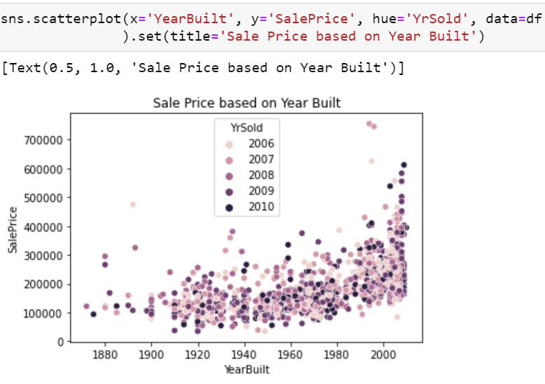
Based on my own prior assumptions and the above heatmap I took a look into YearBuilt due to its 52% correlation. I expected that the year a house was built would have a factor in the overall price of a home.

Experiment 1: Pre-Processing

Dropping variables with null values reduces our overall columns to 62.

Experiment 1: Modeling & Evaluating

For my first experiment, I will be looking into my previous idea of Year Built and Sale Price. Below I am splitting my dataset into training and testing sets. With my training sets, I am able to use Linear Regression to find the coefficient and intercept which can be used to fill in the y = mx + b equation. "m" is the coefficient and "b" is the intercept. The "x" value can be filled in by any year a house was built to give a predicted Sale Price based on the year built.

Based on our coefficient and intercept values we can determine what the sale price should be based on the datasets. For each year after a house is built, we see an increase of $1,343. For example, these two predict values for a house built in 1980 compared to 2020 are $191,469 to $245,194

Here is a similar scatterplot shown above but shown with its line of best fit to show the positive scale with increased years

Experiment 2

For experiment 2 I will be looking into OverallQual due to it being the highest correlation at 79% to SalePrice.

Based on the pattern of the scatter plot graph you can see a distinct positive increase with the increase in the overall quality of the house. Below is a better representation of the positive linear regression based on the line of best fit.

Experiment 3

Lastly, I will look at GrLivArea since it is the second highest correlation at 71% to SalePrice.

Here again, is the same graph but with its regression line shown in black. We can see an even larger positive relationship here based on how steep the line is.

Impact Section

I believe my findings to have a positive impact on the housing market. Homeowners looking to sell their homes can have a better understanding of what drives prices up and down. This may also help individuals who are searching to buy houses. Understanding when a home with positive features like Ground Live Area, Overall Quality, and Year Built is being sold underprice can be a good steal at the time.

Conclusion

Overall, if you have certain variables of a house you can predict its price to an extent. There are still other factors that can also play a role that isn't available with this dataset. Distance from the closest schools, markets, stores, or shopping centers can play a big role in the price. Also houses with a better landscape like vacation homes with beachfront property or mountain lodges can also be highly valued due to location.